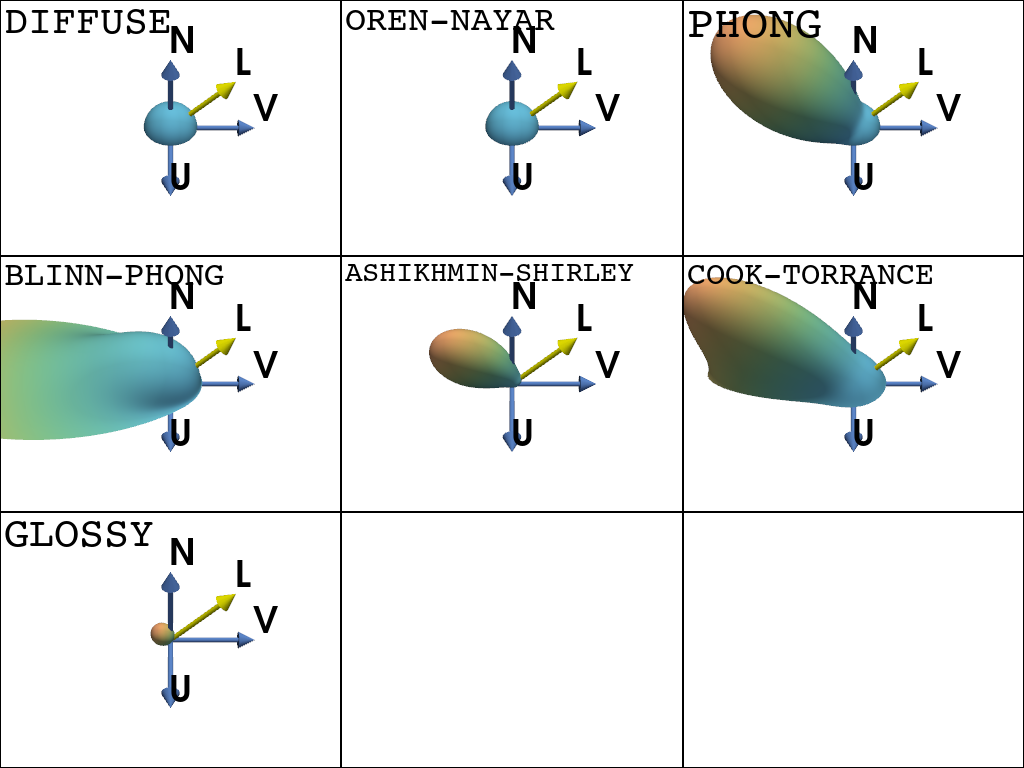
BRDFs in Action

Plotting BRDF kernels and their rendered results

import matplotlib.pyplot as plt
import numpy as np
import pyvista as pv
from PIL import Image

import mirage as mr
import mirage.vis as mrv

brdfs = [
    mr.Brdf('diffuse', 0.5, 0.0, 0),
    mr.Brdf('oren-nayar', 0.5, 0.0, 0),
    mr.Brdf('phong', 0.5, 0.5, 5),
    mr.Brdf('blinn-phong', 0.5, 0.5, 5),
    mr.Brdf('ashikhmin-shirley', 0.5, 0.5, 15),
    mr.Brdf('cook-torrance', 0.5, 0.5, 0.3),
    mr.Brdf('glossy', 0.5, 0.5, 0.9),
]

num = 200
pl_shape = (3, 3)
arrow_scale = 0.5
el_space, az_space = np.linspace(0.1, np.pi / 2, num), np.linspace(0, 2 * np.pi, num)
el_grid, az_grid = np.meshgrid(el_space, az_space)

Now we can iterate through a range of specular exponents and BRDFs to visualize how the BRDF varies

pl = pv.Plotter(shape=pl_shape)
pl.set_background('white')
for i, brdf in enumerate(brdfs):
    (xx, yy, zz) = mr.sph_to_cart(az_grid, el_grid, 0 * el_grid + 1)
    O = np.hstack(
        (
            xx.reshape(((num**2, 1))),
            yy.reshape(((num**2, 1))),
            zz.reshape(((num**2, 1))),
        )
    )
    L = mr.hat(np.tile(np.array([[0, 1, 1]]), (num**2, 1)))
    N = mr.hat(np.tile(np.array([[0, 0, 1]]), (num**2, 1)))
    b = brdf.eval(L, O, N).reshape(xx.shape)
    mesh = pv.StructuredGrid(xx * b, yy * b, zz * b)
    pl.subplot(i // 3, i % 3)
    pl.add_text(f'{brdf.name.upper()}', font_size=18, font='courier', color='black')
    pl.add_mesh(
        mesh,
        scalars=b.T.flatten(),
        show_scalar_bar=False,
        cmap='isolum',
        smooth_shading=True,
    )
    mrv.plot_basis(
        pl, np.eye(3), color='cornflowerblue', labels=['U', 'V', 'N'], scale=arrow_scale
    )
    mrv.plot_arrow(
        pl,
        origin=[0, 0, 0],
        direction=L[0, :],
        scale=arrow_scale,
        color='yellow',
        label='L',
    )

pl.link_views()
pl.camera.position = (2.0, 0.0, 2.0)
pl.camera.focal_point = (0.0, 0.0, 0.0)
pl.show()

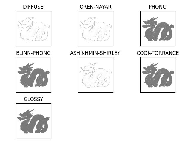
Plotting rendered result with the same BRDFs

ovb = mr.hat(np.tile(np.array([[-1.0, 0.0, 0.5]]), (1, 1)))
svb = mr.hat(np.tile(np.array([[-0.5, 0.0, 0.5]]), (1, 1)))

for i, brdf in enumerate(brdfs):
    mr.run_light_curve_engine(
        brdf, 'stanford_dragon.obj', svb, ovb, save_imgs=True, instances=1
    )
    plt.subplot(*pl_shape, i + 1)
    im = np.asarray(Image.open('out/frame1.png'))
    plt.imshow(im[:, :, 0], cmap='gray', alpha=(im[:, :, 1] > 0).astype(np.float32))
    plt.xticks([])
    plt.yticks([])
    plt.title(brdf.name.upper())
plt.tight_layout()
plt.show()