Earth Albedo BRDF

Modeling the incident radiation at a spacecraft due to reflected sunlight from the Earth

Useful papers not cited below: Kuvyrkin 2016 Strahler 1999

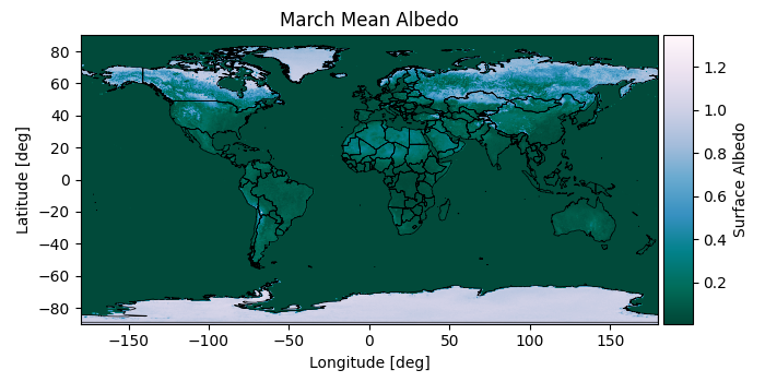
Let’s first load the coefficient arrays \(f_{iso}\), \(f_{geo}\), and \(f_{vol}\) from file

import matplotlib as mpl
import matplotlib.pyplot as plt
import numpy as np

import mirage as mr
import mirage.vis as mrv

save_dict = mr.load_albedo_file()
fiso_map = np.array(save_dict['fiso_map'])
fgeo_map = np.array(save_dict['fgeo_map'])
fvol_map = np.array(save_dict['fvol_map'])
lat_geod_grid = np.array(save_dict['lat_geod_grid'])
lon_grid = np.array(save_dict['lon_grid'])
lat_geod_space = lat_geod_grid[:, 0]
lon_space = lon_grid[0, :]
mapshape = lon_grid.shape

The surface BRDF function in Blanc 2014

pws = (
    lambda ts, fiso, fgeo, fvol: fiso
    + fvol * (-0.007574 - 0.070987 * ts**2 + 0.307588 * ts**3)
    + fgeo * (-1.284909 - 0.166314 * ts**2 + 0.041840 * ts**3)
)
pbs = lambda ts, fiso, fgeo, fvol: fiso + 0.189184 * fvol - 1.377622 * fgeo
albedo = lambda ts, fiso, fgeo, fvol: 0.5 * pws(ts, fiso, fgeo, fvol) + 0.5 * pbs(
    ts, fiso, fgeo, fvol
)

Now we define the date to evaluate the reflected albedo irradiance at and the ECEF position of the satellite

date = mr.utc(2022, 6, 23, 5, 53, 0)
datestr = f'{date.strftime("%Y-%m-%d %H:%M:%S")} UTC'
sat_pos_ecef = (mr.AstroConstants.earth_r_eq + 4e4) * mr.hat(np.array([[1, 1, 0]]))

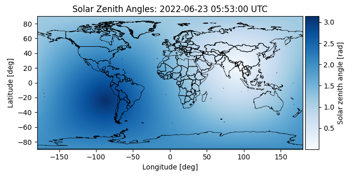
Now we identify all the useful geometry: the ECEF positions of the grid cells, the Sun vector, the solar zenith angle at each grid cell, and the albedo at each point

ecef_grid = mr.lla_to_itrf(
    lat_geod=lat_geod_grid.flatten(),
    lon=lon_grid.flatten(),
    alt_km=0 * lon_grid.flatten(),
)
j2000_to_itrf_rotm = mr.itrf_to_j2000(date).T
sun_ecef_hat = (j2000_to_itrf_rotm @ mr.hat(mr.sun(date)).T).T
sun_dir = np.tile(sun_ecef_hat, (ecef_grid.shape[0], 1))
solar_zenith = mr.angle_between_vecs(ecef_grid, sun_dir)
solar_zenith_grid = solar_zenith.reshape(mapshape)
albedo_grid = albedo(solar_zenith_grid, fiso_map, fgeo_map, fvol_map)

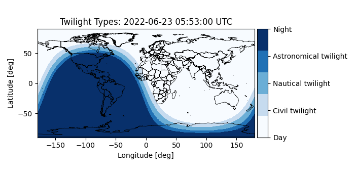
For fun, let’s classify the types of twilight to plot later

solar_type_grid = np.zeros_like(solar_zenith_grid)
solar_type_grid[
    (solar_zenith_grid > np.pi / 2) & (solar_zenith_grid < np.pi / 2 + np.deg2rad(18))
] = 3
# Astronomical twilight
solar_type_grid[
    (solar_zenith_grid > np.pi / 2) & (solar_zenith_grid < np.pi / 2 + np.deg2rad(12))
] = 2
# Nautical twilight
solar_type_grid[
    (solar_zenith_grid > np.pi / 2) & (solar_zenith_grid < np.pi / 2 + np.deg2rad(6))
] = 1
# Civil twilight
solar_type_grid[solar_zenith_grid > np.pi / 2 + np.deg2rad(16)] = 4
# Night

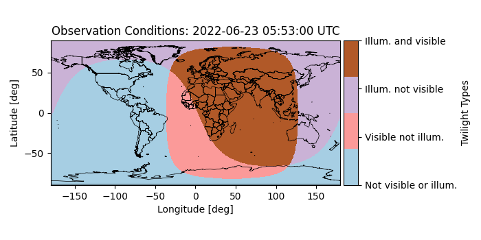
Computing which grid cells are visible from the satellite

surf_to_sat = sat_pos_ecef - ecef_grid
surf_to_sat_dir = mr.hat(surf_to_sat)
surf_to_sat_rmag_m_grid = 1e3 * mr.vecnorm(surf_to_sat).reshape(mapshape)
tosat_to_normal_ang = mr.angle_between_vecs(ecef_grid, surf_to_sat_dir)
tosat_to_normal_grid = tosat_to_normal_ang.reshape(mapshape)
pt_visible_from_sat = tosat_to_normal_grid < np.pi / 2

# Visible and illuminated points
ill_and_vis = pt_visible_from_sat & (solar_type_grid == 0)
brdf_to_brightness = np.cos(solar_zenith_grid) * np.cos(tosat_to_normal_grid)
loss_at_surf_diffuse = brdf_to_brightness * ill_and_vis * albedo_grid
is_ocean = np.abs(albedo_grid - albedo_grid[0, 0]) < 1e-8
loss_at_surface_specular = (
    mr.brdf_phong(sun_dir, surf_to_sat_dir, mr.hat(ecef_grid), 0, 0.4, 10).reshape(
        mapshape
    )
    * is_ocean
    * brdf_to_brightness
)

obs_type_grid = np.zeros_like(solar_zenith_grid)
obs_type_grid[pt_visible_from_sat] = 1
obs_type_grid[(solar_type_grid == 0) & ~pt_visible_from_sat] = 2
obs_type_grid[ill_and_vis] = 3

Computes the areas of each grid cell

dp, dt = (
    lat_geod_space[1] - lat_geod_space[0],
    lon_space[1] - lon_space[0],
)
cell_area_grid = np.tile(
    np.array(
        [mr.lat_lon_cell_area((p + dp, p), (0, dt)) for p in lat_geod_space]
    ).reshape(-1, 1),
    (1, lon_space.size),
)

Computing Lambertian reflection (for the land) and Phong reflection (for the ocean) from each grid cell

rmag_loss_grid = 1 / surf_to_sat_rmag_m_grid**2
irrad_from_surf = (
    mr.total_solar_irradiance_at_dates(date)
    * rmag_loss_grid
    * cell_area_grid
    * (loss_at_surf_diffuse + loss_at_surface_specular)
)
print(f'{np.sum(irrad_from_surf):.2e}')

6.48e+00

Let’s compare with the implementation in the pyspaceaware package

mr.tic()
alb_irrad = mr.albedo_irradiance(date, sat_pos_ecef)
mr.toc()
print(f'{alb_irrad:.2e}')

Elapsed time: 1.79e-01 seconds
6.48e+00

Defining a few useful functions to simplify the plotting process

bcmap = 'PiYG'

Plotting the albedo across the grid

mrv.plot_map_with_grid(
    albedo_grid, 'March Mean Albedo', 'Surface Albedo', cmap='PuBuGn_r', borders=True
)
plt.show()

Plotting the solar zenith angle

mrv.plot_map_with_grid(
    solar_zenith_grid,
    f'Solar Zenith Angles: {datestr}',
    'Solar zenith angle [rad]',
    cmap='Blues',
    borders=True,
)
plt.show()

Plotting the twilight types

mrv.plot_map_with_grid(
    solar_type_grid,
    f'Twilight Types: {datestr}',
    '',
    cmap=mpl.colormaps['Blues'].resampled(5),
    borders=True,
    cbar_tick_labels=[
        'Day',
        'Civil twilight',
        'Nautical twilight',
        'Astronomical twilight',
        'Night',
    ],
)
plt.show()

Plotting grid cell visibility and illumination conditions

mrv.plot_map_with_grid(
    obs_type_grid,
    f'Observation Conditions: {datestr}',
    'Twilight Types',
    cmap=mpl.colormaps['Paired'].resampled(4),
    borders=True,
    interpolation='nearest',
    cbar_tick_labels=[
        'Not visible or illum.',
        'Visible not illum.',
        'Illum. not visible',
        'Illum. and visible',
    ],
)
plt.show()

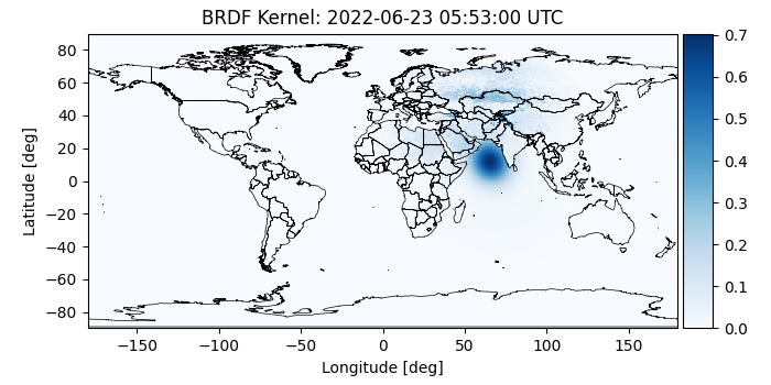
BRDF kernel values at each point

mrv.plot_map_with_grid(
    loss_at_surf_diffuse + loss_at_surface_specular,
    f'BRDF Kernel: {datestr}',
    '',
    cmap='Blues',
    borders=True,
    interpolation='nearest',
)
plt.show()

Plotting the areas of each grid cell

mrv.plot_map_with_grid(
    cell_area_grid,
    f'Cell Areas: {datestr}',
    '$[m^2]$',
    cmap='Blues',
    borders=True,
    interpolation='nearest',
)
plt.show()

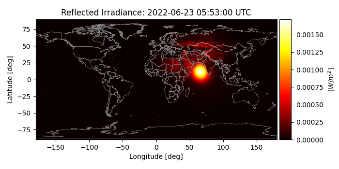
Plotting the irradiance from each grid cell

mrv.plot_map_with_grid(
    irrad_from_surf,
    f'Reflected Irradiance: {datestr}',
    r'$\left[W/m^2\right]$',
    cmap='hot',
    borders=True,
    border_color='gray',
    interpolation='nearest',
)
plt.show()