Random Sphere Point Statistics

How does the geometry of the \(n\)-sphere impact the statistics of uniform randomly sampled points on the surface?

import matplotlib.pyplot as plt
import numpy as np
from scipy.optimize import fsolve
from sympy import integrate, pi, sin, symbols

import mirage as mr

t = symbols('t')
f_theta = 2 / pi * sin(t / 2) ** 2
F_theta = integrate(f_theta, t)
assert integrate(f_theta, (t, 0, pi)) == 1
pdf = lambda theta: 2 / np.pi * np.sin(theta / 2) ** 2
cdf = lambda theta: 2 * (theta / 2 - np.sin(theta / 2) * np.cos(theta / 2)) / np.pi

# h = lambda p, theta: 1 / np.sqrt(np.pi) * gamma(p/2)/gamma((p-1)/2) * np.sin(theta) ** (p-2)

small_bound = 1

print('For the 3-sphere')
E_theta = float(integrate(t * f_theta, (t, 0, pi)).evalf())
Var_theta = float(integrate(t**2 * f_theta, (t, 0, pi)).evalf()) - E_theta**2
print('Expected value [deg]: ', np.rad2deg(E_theta))  # np.pi/2 + 2/np.pi radians
print('Stdev [deg]: ', np.sqrt(Var_theta * 180**2 / np.pi**2))
print(
    'Median value [deg]: ',
    fsolve(lambda x: cdf(np.deg2rad(x)) - 0.5, np.rad2deg(E_theta))[0],
)
print('Probability less than 90 degrees: ', cdf(np.deg2rad(90)))
print(f'Probability less than {small_bound} degrees: ', cdf(np.deg2rad(small_bound)))

n = int(1e6 + 1)
q = mr.rand_quaternions(n)
ang = np.sort(np.abs(mr.quat_ang(q[1:], q[0])))

print('Numerical mean [deg]: ', np.rad2deg(np.mean(ang)))
print('Numerical median [deg]: ', np.rad2deg(np.median(ang)))
print('Numerical std [deg]: ', np.rad2deg(np.std(ang)))

plt.figure()
plt.hist(ang, bins=100, density=True, alpha=0.5, label='Numerical')
plt.plot(ang, pdf(ang), label='Analytical')
plt.xlabel('Angle between two random samples [rad]')
plt.ylabel('Probability density')
plt.title(r'Error pdf on $S^3$')
plt.legend()
plt.grid()
plt.tight_layout()
plt.show()

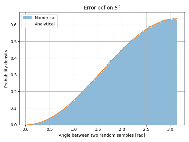
For the 3-sphere
Expected value [deg]:  126.47562611124161
Stdev [deg]:  37.00714390212934
Median value [deg]:  132.3464588340929
Probability less than 90 degrees:  0.1816901138162093
Probability less than 1 degrees:  2.8204887058521865e-07
Numerical mean [deg]:  126.48542517386812
Numerical median [deg]:  132.28011819975205
Numerical std [deg]:  36.95381256062406

Doing the same for the 2-sphere

print('For the 2-sphere')
pts = mr.rand_unit_vectors(n)
ang = np.sort(mr.angle_between_vecs(pts[1:], pts[0]).flatten())

f_theta = 1 / 2 * sin(t)
F_theta = integrate(f_theta, t) + 1 / 2
pdf = lambda theta: 1 / 2 * np.sin(theta)
cdf = lambda theta: -1 / 2 * np.cos(theta) + 1 / 2
assert integrate(f_theta, (t, 0, pi)) == 1.0

E_theta = float(integrate(t * f_theta, (t, 0, pi)).evalf())
Var_theta = float(integrate(t**2 * f_theta, (t, 0, pi)).evalf()) - E_theta**2
print('Expected value [deg]: ', np.rad2deg(E_theta))
print('Stdev [deg]: ', np.sqrt(Var_theta * 180**2 / np.pi**2))
print(
    'Median value [deg]: ',
    fsolve(lambda x: cdf(np.deg2rad(x)) - 0.5, np.rad2deg(E_theta))[0],
)
print('Probability less than 90 degrees: ', cdf(np.deg2rad(90)))
print(f'Probability less than {small_bound} degrees: ', cdf(np.deg2rad(small_bound)))

print('Numerical mean [deg]: ', np.rad2deg(np.mean(ang)))
print('Numerical median [deg]: ', np.rad2deg(np.median(ang)))
print('Numerical std [deg]: ', np.rad2deg(np.std(ang)))

# for small angles, say 1 deg, it is 270x less likely to sample a unit vector pair within that margin on the 3-sphere than the 2-sphere.
# if those angles get 10x closer, it is now 2700x less likely on the 3-sphere

plt.figure()
plt.hist(ang, bins=100, density=True, alpha=0.5, label='Numerical')
plt.plot(ang, pdf(ang), label='Analytical')
plt.xlabel('Angle between two random samples [rad]')
plt.ylabel('Probability density')
plt.title(r'Error pdf on $S^2$')
plt.legend()
plt.grid()
plt.tight_layout()

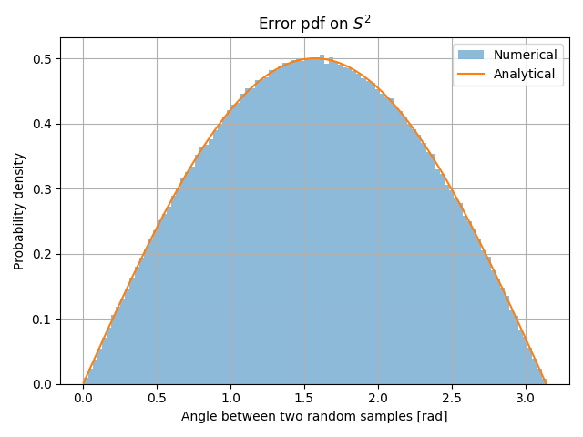
For the 2-sphere
Expected value [deg]:  90.0
Stdev [deg]:  39.17125604287554
Median value [deg]:  90.0
Probability less than 90 degrees:  0.49999999999999994
Probability less than 1 degrees:  7.615242180436521e-05
Numerical mean [deg]:  90.01015092929406
Numerical median [deg]:  89.9641804362087
Numerical std [deg]:  39.15619992346243

And for the 1-sphere

ang = np.sort(np.pi * np.random.rand(n))

f_theta = 1 / pi
F_theta = 1 / pi * t

pdf = lambda theta: np.full_like(theta, 1 / np.pi)
cdf = lambda theta: 1 / np.pi * theta
assert integrate(f_theta, (t, 0, pi)) == 1

E_theta = float(integrate(t * f_theta, (t, 0, pi)).evalf())
Var_theta = float(integrate(t**2 * f_theta, (t, 0, pi)).evalf()) - E_theta**2
print('Expected value [deg]: ', np.rad2deg(E_theta))
print('Stdev [deg]: ', np.sqrt(Var_theta * 180**2 / np.pi**2))
print(
    'Median value [deg]: ',
    fsolve(lambda x: cdf(np.deg2rad(x)) - 0.5, np.rad2deg(E_theta))[0],
)
print('Probability less than 90 degrees: ', cdf(np.deg2rad(90)))
print(f'Probability less than {small_bound} degrees: ', cdf(np.deg2rad(small_bound)))

print('Numerical mean [deg]: ', np.rad2deg(np.mean(ang)))
print('Numerical median [deg]: ', np.rad2deg(np.median(ang)))
print('Numerical std [deg]: ', np.rad2deg(np.std(ang)))

plt.figure()
plt.hist(ang, bins=100, density=True, alpha=0.5, label='Numerical')
plt.plot(ang, pdf(ang), label='Analytical')
plt.xlabel('Angle between two random samples [rad]')
plt.ylabel('Probability density')
plt.title(r'Error pdf on $S^1$')
plt.legend()
plt.grid()
plt.tight_layout()
plt.show()

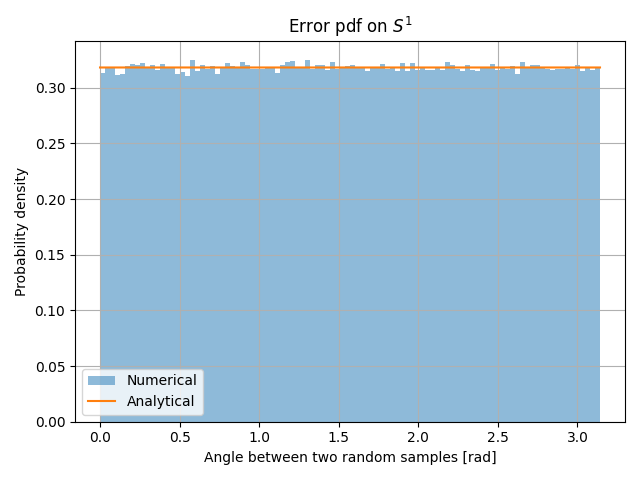
Expected value [deg]:  90.0
Stdev [deg]:  51.96152422706632
Median value [deg]:  90.0
Probability less than 90 degrees:  0.5
Probability less than 1 degrees:  0.005555555555555556
Numerical mean [deg]:  89.9967762112473
Numerical median [deg]:  89.93947499969207
Numerical std [deg]:  51.91728320024072