Signal-to-Noise Ratio (SNR)

Investigating the SNR applied to CCD images

import matplotlib.pyplot as plt
import numpy as np

import mirage as mr
import mirage.vis as mrv


def ccd_snr(signal_grid: np.ndarray, noise_grid: np.ndarray) -> float:
    return np.sum(signal_grid) / np.sqrt(np.sum(signal_grid) + np.sum(noise_grid))


telescope = mr.Telescope(preset='pogs')
telescope.sensor_pixels = np.array([50, 50])
telescope.pixel_scale = 0.2

obj_pos = (
    telescope.sensor_pixels[0] // 2 - 0.5,
    telescope.sensor_pixels[1] // 2 - 0.5,
)
x_pix, y_pix = np.meshgrid(
    np.arange(telescope.sensor_pixels[0]), np.arange(telescope.sensor_pixels[1])
)
r_dist = np.sqrt((x_pix - obj_pos[0]) ** 2 + (y_pix - obj_pos[1]) ** 2)
theta_grid_rad = mr.dms_to_rad(0, 0, r_dist * telescope.pixel_scale)

dt = 0.3
c_all = 1e4 * dt
airy_pattern = telescope.gaussian_diffraction_pattern(c_all, theta_grid_rad)
print(f'Airy disk volume: {np.sum(airy_pattern):.4f}')

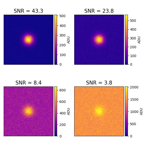
plt.figure(figsize=(6, 6))

br_levels = [1e1, 1e2, 1e3, 5e3]
for i, c_background in enumerate(br_levels):
    c_background *= dt
    adu_grid = np.random.poisson(lam=airy_pattern + c_background).astype(float)

    two_sigma_pixel_width = (
        3 * telescope.fwhm / (2 * np.sqrt(2 * np.log(2))) / telescope.pixel_scale
    )
    two_sigma_pixel_area = np.pi * two_sigma_pixel_width**2

    is_obj = r_dist < two_sigma_pixel_width
    total_noise_and_signal = np.sum(adu_grid[is_obj])
    total_signal = np.sum(airy_pattern[is_obj])

    snr1 = 0.838 * c_all / np.sqrt(0.838 * c_all + two_sigma_pixel_area * c_background)
    snr2 = ccd_snr(airy_pattern[is_obj], adu_grid[is_obj] - airy_pattern[is_obj])

    print(f'Background mean: {c_background}')
    print(f'SNR from means: {snr1:.2f} \nSNR from samples: {snr2:.2f}')

    plt.subplot(2, 2, i + 1)
    plt.imshow(
        adu_grid,
        cmap='plasma',
        extent=[x_pix.min(), x_pix.max(), y_pix.min(), y_pix.max()],
    )
    mrv.texit(f'SNR = {snr1:.1f}', '', '', grid=False)
    plt.xticks([])
    plt.yticks([])
    plt.clim(0, np.max(adu_grid))
    plt.colorbar(cax=mrv.get_cbar_ax(), label='ADU')
plt.tight_layout()
plt.show()

Airy disk volume: 33076.2815
Background mean: 3.0
SNR from means: 43.28
SNR from samples: 178.71
Background mean: 30.0
SNR from means: 23.84
SNR from samples: 160.52
Background mean: 300.0
SNR from means: 8.45
SNR from samples: 95.31
Background mean: 1500.0
SNR from means: 3.82
SNR from samples: 48.28

Investigating the effect of integration time on SNR

dts = np.linspace(0.1, 10, 40)
c_background = 1e2
c_all = 1e3
snrs = []

for dt in dts:
    airy_pattern = telescope.gaussian_diffraction_pattern(c_all * dt, theta_grid_rad)
    adu_grid = np.random.poisson(lam=airy_pattern + c_background * dt).astype(float)

    two_sigma_pixel_width = (
        3 * telescope.fwhm / (2 * np.sqrt(2 * np.log(2))) / telescope.pixel_scale
    )
    two_sigma_pixel_area = np.pi * two_sigma_pixel_width**2

    is_obj = r_dist < two_sigma_pixel_width
    snrs.append(ccd_snr(airy_pattern[is_obj], adu_grid[is_obj] - airy_pattern[is_obj]))

snrs = np.array(snrs)

# finding the slope of the log-log plot
m, b = np.polyfit(np.log10(dts), np.log10(snrs), 1)
print(f'SNR ~ x^{m:.2f}')

plt.plot(dts, snrs)
plt.scatter(dts, snrs)
mrv.texit('', 'Integration Time (s)', 'SNR', ['$\sqrt{\Delta t} + \mathrm{SNR}_0$'])
plt.tight_layout()
plt.show()

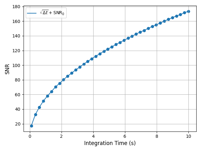
SNR ~ x^0.50