Solar Spectrum

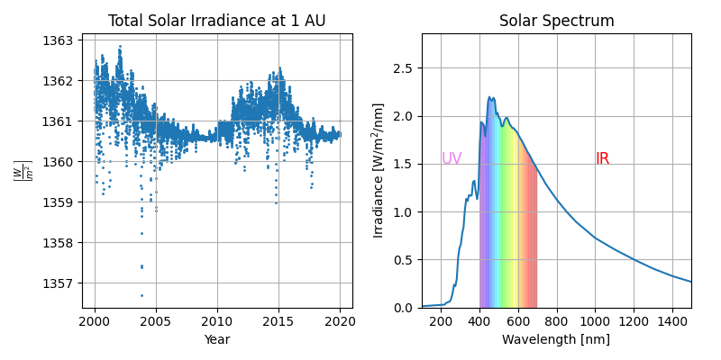
Plots of the solar irradiance spectrum and the total solar irradiance.

import matplotlib.pyplot as plt
import numpy as np
from terrainman import TsiDataHandler

import mirage as mr
import mirage.vis as mrv

The solar spectrum and irradiance at Earth

date = mr.utc(2000, 1, 1, 12)
dates, epsecs = mr.date_arange(
    date, date + mr.years(20), mr.days(1), return_epsecs=True
)
epyrs = epsecs / 86400 / 365.25

The terrainman.TsiDataHandler class deals with downloading the relevant netCDF4 files from This NOAA server. Outside of the interval covered by this dataset (1882-current_year) \(1361 \frac{W}{m^2}\) is used as a default.

tsi_dh = TsiDataHandler()
mr.tic()
sc_at_one_au = tsi_dh.eval(dates)
mr.toc()

earth_to_sun = mr.sun(dates)
earth_to_sun_dist_km = mr.vecnorm(earth_to_sun).flatten()
earth_to_sun_dist_au = earth_to_sun_dist_km / mr.AstroConstants.au_to_km

File not found in storage, proceeding to download...
Downloading tsi_v02r01_daily_s20170101_e20171231_c20180227.nc...
Using: https://www.ncei.noaa.gov/data/total-solar-irradiance/access/daily/tsi_v02r01_daily_s20170101_e20171231_c20180227.nc
File not found in storage, proceeding to download...
Downloading tsi_v02r01_daily_s20180101_e20181231_c20190409.nc...
Using: https://www.ncei.noaa.gov/data/total-solar-irradiance/access/daily/tsi_v02r01_daily_s20180101_e20181231_c20190409.nc
File not found in storage, proceeding to download...
Downloading tsi_v02r01_daily_s20190101_e20191231_c20200226.nc...
Using: https://www.ncei.noaa.gov/data/total-solar-irradiance/access/daily/tsi_v02r01_daily_s20190101_e20191231_c20200226.nc
Elapsed time: 2.12e+00 seconds

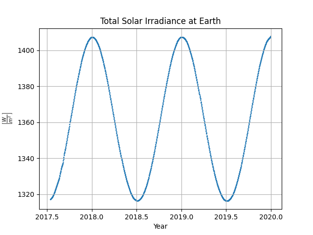
With this distance information, we can augment the Total Solar Irradiance plot to show the actual irradiance felt by a shell at Earth’s instantaneous orbital radius. We can do this by noting that doubling the radius of a sphere squares its area, so we just have to divide by the square of the earth_to_sun_dist_au

plt.figure(figsize=(8, 4))
plt.subplot(1, 2, 1)
sc_at_earth_radius = sc_at_one_au / earth_to_sun_dist_au**2
ax1 = plt.gca()
ax1.scatter(epyrs + 2000, sc_at_one_au, s=1, color='C0')
ax1.set_ylabel(r'$\left[\frac{W}{m^2}\right]$')
ax1.set_xlabel('Year')
plt.title('Total Solar Irradiance at 1 AU')
plt.grid()

plt.subplot(1, 2, 2)

lambdas = np.linspace(100, 1500, 200)

solar_spectrum = mr.sun_spectrum(lambdas)
plt.plot(lambdas, solar_spectrum)
mrv.plot_visible_band(lambdas, solar_spectrum)
# label IR and UV
plt.xlim([np.min(lambdas), np.max(lambdas)])
plt.ylim([0, 1.3 * np.max(solar_spectrum)])
plt.text(1000, 1.5, 'IR', color='r', fontsize=12)
plt.text(200, 1.5, 'UV', color='violet', fontsize=12)

plt.title('Solar Spectrum')
plt.xlabel('Wavelength [nm]')
plt.ylabel('Irradiance [W/m$^2$/nm]')
plt.grid()
plt.tight_layout()
plt.show()

True irradiance at Earth

plt.scatter(epyrs[-900:] + 2000, sc_at_earth_radius[-900:], s=1)
plt.ylabel(r'$\left[\frac{W}{m^2}\right]$')
plt.xlabel('Year')
plt.title('Total Solar Irradiance at Earth')
plt.grid()
plt.show()