Skellam Distribution

The difference of two Poisson distributions

import matplotlib.pyplot as plt
import numpy as np
from scipy.special import iv

n = int(1e6)  # samples
lams = [10, 4]
s1 = np.random.poisson(lam=lams[0], size=n)
s2 = np.random.poisson(lam=lams[1], size=n)

p_skellam = (
    lambda x, lam1, lam2: np.exp(-lam1 - lam2)
    * (lam1 / lam2) ** (x / 2)
    * iv(x, 2 * np.sqrt(lam1 * lam2))
)
xs = np.linspace(-20, 20)
pxs = p_skellam(xs, *lams)
diff = s1 - s2

print(f'Numerical  mean: {diff.mean():.3f}')
print(f'Analytical mean: {lams[0]-lams[1]:.3f}\n')
print(f'Numerical  variance: {diff.var():.3f}')
print(f'Analytical variance: {lams[0]+lams[1]:.3f}')

Numerical  mean: 6.002
Analytical mean: 6.000

Numerical  variance: 13.984
Analytical variance: 14.000

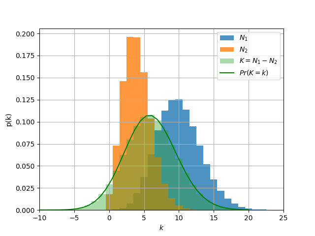
Let’s plot these sampled random variables as well as the expected distribution of their difference

plt.hist(
    s1,
    bins=range(s1.min(), s1.max() + 1),
    alpha=0.8,
    density=True,
    align='left',
    label='$N_1$',
)
plt.hist(
    s2,
    bins=range(s1.min(), s1.max() + 1),
    alpha=0.8,
    density=True,
    align='left',
    label='$N_2$',
)
plt.hist(
    diff,
    bins=range(diff.min(), diff.max() + 1),
    alpha=0.4,
    density=True,
    align='left',
    label='$K=N_1-N_2$',
)
plt.plot(xs, pxs, color='g', label='$Pr(K=k)$')
plt.xlabel('$k$')
plt.ylabel('p(k)')
plt.legend()
plt.xlim(-10, 25)
plt.grid()
plt.show()