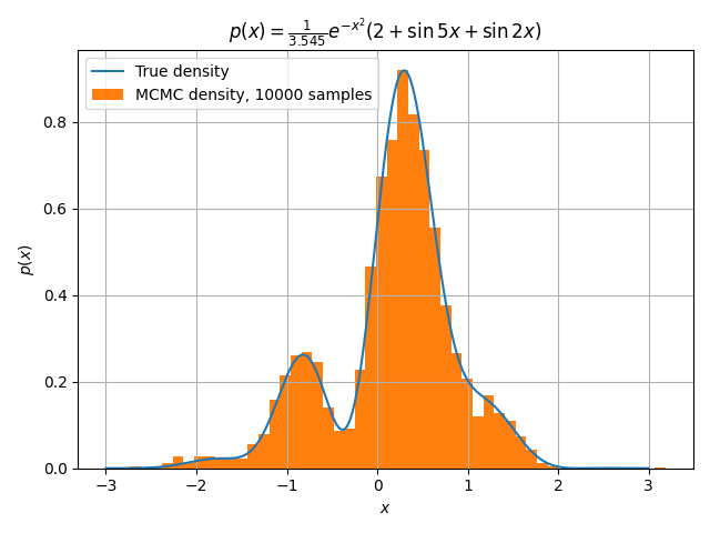
Metropolis Hastings MCMC

Markov Chain Monte Carlo approximation of an unknown probability density

import matplotlib.pyplot as plt
import numpy as np

px = lambda x: np.exp(-(x**2)) * (2 + np.sin(5 * x) + np.sin(2 * x))

sigma = 1.0
q = (
    lambda loc, x: 1
    / (np.sqrt(2 * np.pi * sigma**2))
    * np.exp(-1 / 2 * (x - loc) ** 2 / sigma**2)
)
q_sampler = lambda x: np.random.normal(loc=x, scale=sigma)

xn = 0.0
n_samples = 10000
burn_in = 200

xns = [xn]
for i in range(n_samples):
    xsn = q_sampler(xn)
    acceptance_probability = min(1, px(xsn) / px(xn))
    if acceptance_probability > np.random.rand():  # if accepted
        xn = xsn
    else:
        pass
    if i >= burn_in:
        xns.append(xn)

x = np.linspace(-3, 3, 1000)
ps = np.trapz(px(x), x)
plt.plot(x, px(x) / ps, label='True density')
plt.hist(xns, bins=50, density=True, label=f'MCMC density, {n_samples} samples')
plt.title(r'$p(x) = \frac{1}{3.545} e^{-x^2}\left(2 + \sin 5x + \sin 2x\right)$')
plt.grid()
plt.legend()
plt.xlabel('$x$')
plt.ylabel('$p(x)$')
plt.tight_layout()
plt.show()