Restricted Circular IOD

import matplotlib.pyplot as plt
import numpy as np
import pyvista as pv
from scipy.optimize import root_scalar

import mirage as mr
import mirage.vis as mrv

First, let’s define a station and a truth object

station = mr.Station()
obj = mr.SpaceObject('cube.obj', identifier=25544)

Now, let’s create two RA/Dec observations of the object

r_lims = [mr.AstroConstants.earth_r_eq, 1e6]
dates = mr.date_linspace(mr.now(), mr.now() + mr.minutes(1), 2)

r_sat_truth = obj.propagate(dates)
r_station = station.j2000_at_dates(dates)
r_station_to_sat_truth = r_sat_truth - r_station
rho_truth = mr.vecnorm(r_station_to_sat_truth)
line_of_sight_truth = mr.hat(r_station_to_sat_truth)

ra_truth, dec_truth = mr.eci_to_ra_dec(line_of_sight_truth)

print(f'ra_truth = {ra_truth} [rad]')
print(f'dec_truth = {dec_truth} [rad]')

ra_truth = [2.18247321 2.1588651 ] [rad]
dec_truth = [-1.25881232 -1.31355334] [rad]

To check our work, we should be able to go in the opposite direction to recover the same satellite position vector

line_of_sight_backwards = mr.ra_dec_to_eci(ra_truth, dec_truth)
assert np.all(
    np.abs(line_of_sight_backwards * rho_truth + r_station - r_sat_truth) < 1e-10
), 'Something went wrong!'

Now, let’s add some noise to our observations

sigma_obs_arcsec = 10.0
sigma_obs_rad = mr.dms_to_rad(0, 0, sigma_obs_arcsec)
ra_obs = ra_truth + np.random.normal(0, sigma_obs_rad, size=ra_truth.shape)
dec_obs = dec_truth + np.random.normal(0, sigma_obs_rad, size=dec_truth.shape)

print(f'ra_obs = {ra_obs} [rad]')
print(f'dec_obs = {dec_obs} [rad]')

ra_obs = [2.18242872 2.15882789] [rad]
dec_obs = [-1.25880856 -1.3134719 ] [rad]

With these observations in hand, we can start to estimate things about the orbit We know that the ranges to the object \(\rho_1\) and \(\rho_2\) are only a function of the semimajor axis \(a\)

lhats = mr.ra_dec_to_eci(ra_obs, dec_obs)
lhat1 = lhats[[0]]
lhat2 = lhats[[1]]
rtopo1 = r_station[[0]]
rtopo2 = r_station[[1]]

rho_1 = lambda a: (
    -mr.dot(lhat1, rtopo1)
    + np.sqrt(mr.dot(lhat1, rtopo1) ** 2 + a**2 - mr.vecnorm(rtopo1) ** 2)
).flatten()
rho_2 = lambda a: (
    -mr.dot(lhat2, rtopo2)
    + np.sqrt(mr.dot(lhat2, rtopo2) ** 2 + a**2 - mr.vecnorm(rtopo2) ** 2)
).flatten()
r_sat_1 = lambda a: rtopo1 + rho_1(a).reshape(-1, 1) * lhat1
r_sat_2 = lambda a: rtopo2 + rho_2(a).reshape(-1, 1) * lhat2
rhat_sat_1 = lambda a: mr.hat(r_sat_1(a))
rhat_sat_2 = lambda a: mr.hat(r_sat_2(a))

We know that a circular orbit has a constant true anomaly rate, equal to the mean motion \(n = \sqrt{\mu/a^3}\) This means that the angle between the true position vectors of the object at the two observation times is equal to the mean motion times the time between the observations

dt = (dates[1] - dates[0]).total_seconds()
c = mr.AstroConstants.speed_of_light_vacuum

phi_cm = lambda a: np.sqrt(mr.AstroConstants.earth_mu / a**3) * (
    dt - rho_2(a) / np.inf + rho_1(a) / np.inf
)

Additionally, the angle between between the position vectors must satisfy the law of cosines

phi_g = lambda a: np.arccos(mr.dot(rhat_sat_1(a), rhat_sat_2(a))).flatten()

For an arbitrary \(a\), the geometry and dynamics of the problem will not produce the same answer! We need to use a root-finding algorithm to find the value of \(a\) that satisfies both equations

sol = root_scalar(lambda a: phi_g(a) - phi_cm(a), bracket=r_lims)
assert sol.converged, 'Something went wrong!'
a_est = sol.root  # The estimated semimajor axis in km

print(f'a_est = {a_est} [km]')

a = np.linspace(r_lims[0], r_lims[1], 1000)

plt.plot(a, phi_g(a).flatten(), label=r'$\phi_g$')
plt.plot(a, phi_cm(a).flatten(), label=r'$\phi_{cm}$')
plt.plot(a_est, phi_g(a_est), 'o', color='black', label=r'$a_{est}$')
plt.xlabel('Semimajor axis [km]')
plt.ylabel('Elapsed Anomaly [rad]')
plt.legend()
plt.grid()
plt.show()

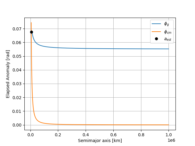
a_est = 6804.522813883358 [km]

Now we can find the estimated position vectors at the two observation times

r_sat_1_est = r_sat_1(a_est)
r_sat_2_est = r_sat_2(a_est)

From orbital mechanics, we know that the angular momentum direction is perpendicular to the orbital plane, and that the cross product of the position and velocity vectors is equal to the angular momentum vector

hhat_est = mr.hat(np.cross(r_sat_1_est, r_sat_2_est))

The velocity vector must be perpendicular to the position vector and the angular momentum vector, with magnitude equal to the circular velocity \(v_c = \sqrt{\mu/a}\)

v_c_est = np.sqrt(mr.AstroConstants.earth_mu / a_est)
vhat_est = mr.hat(np.cross(hhat_est, r_sat_1_est))

v_est = v_c_est * vhat_est

print(f'v_est = {v_est} [km/s]')

v_est = [[ 4.07573796 -4.80140163 -4.34898295]] [km/s]

Let’s see how well the estimated orbit matches the measurements

lhat_synth1 = mr.hat(r_sat_1_est - r_station[[0]])
lhat_synth2 = mr.hat(r_sat_2_est - r_station[[1]])

ra_synth1, dec_synth1 = mr.eci_to_ra_dec(lhat_synth1)
ra_synth2, dec_synth2 = mr.eci_to_ra_dec(lhat_synth2)

print(f'ra_error1 = {ra_synth1 - ra_obs[0]} [rad]')
print(f'dec_error1 = {dec_synth1 - dec_obs[0]} [rad]')
print(f'ra_error2 = {ra_synth2 - ra_obs[1]} [rad]')
print(f'dec_error2 = {dec_synth2 - dec_obs[1]} [rad]')

ra_error1 = [0.] [rad]
dec_error1 = [0.] [rad]
ra_error2 = [4.4408921e-16] [rad]
dec_error2 = [0.] [rad]

Plotting the orbits

dates_plot = mr.date_linspace(mr.now(), mr.now() + mr.hours(24), 1000)

rv0 = np.hstack([r_sat_1_est, v_est])
r_est_propagated = mr.integrate_orbit_dynamics(rv0, dates_plot)[:, :3]
r_true_propagated = obj.propagate(dates_plot)

print(
    f'maximum position error = {mr.vecnorm(r_est_propagated - r_true_propagated).max()} [km]'
)

pl = pv.Plotter(window_size=(2500, 1400))
mrv.plot3(pl, r_est_propagated, color='magenta', lighting=False, line_width=5)
mrv.plot3(pl, r_true_propagated, color='lime', lighting=False, line_width=5)

mrv.plot_earth(pl, date=mr.now())
pl.show()

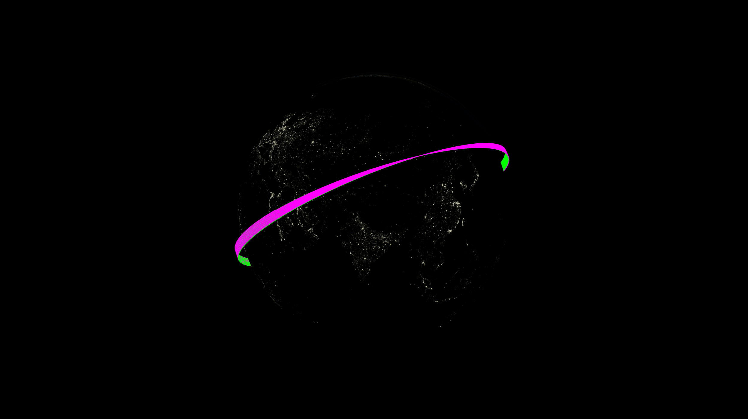
maximum position error = 1723.8576928098541 [km]

We could solve for other orbital elements: The inclination of the orbit is the angle between the angular momentum vector and the inertial z-axis

i_est = mr.angle_between_vecs(hhat_est, np.array([0, 0, 1])).squeeze()

print(f'i_est = {i_est} [rad]')

i_est = 0.9003080879195137 [rad]

The cross product of the inertial z-axis with angular momentum vector is the ascending node vector. The right ascension of the ascending node is the angle between the ascending node vector and the inertial x-axis

Omega_hat_est = mr.hat(np.cross(np.array([0, 0, 1]), hhat_est))
Omega_est = mr.angle_between_vecs(Omega_hat_est, np.array([1, 0, 0])).squeeze()
print(f'Omega_est = {Omega_est} [rad]')

Omega_est = 0.2874384404251377 [rad]

The argument of latitude is the angle between the ascending node vector and the position vector at the first observation time

u_est = mr.angle_between_vecs(Omega_hat_est, r_sat_1_est).squeeze()
print(f'u_est = {u_est} [rad]')

u_est = 2.3821470202291364 [rad]