Convolution for Streaks

import matplotlib.pyplot as plt
import numpy as np

import mirage as mr
import mirage.vis as mrv

telescope = mr.Telescope(preset='pogs')
telescope.sensor_pixels = np.array([40, 40])
telescope.pixel_scale = 0.05
telescope.fwhm = (
    telescope.airy_disk_fwhm(550.0) * mr.AstroConstants.rad_to_arcsecond
)  # arcseconds

c_all = 10
obj_pos = (20, 20)
x_pix, y_pix = np.meshgrid(
    np.arange(telescope.sensor_pixels[0]), np.arange(telescope.sensor_pixels[1])
)
r_dist = np.sqrt((x_pix - obj_pos[0] + 0.5) ** 2 + (y_pix - obj_pos[1] + 0.5) ** 2)
theta_grid_rad = mr.dms_to_rad(0, 0, r_dist * telescope.pixel_scale)

gaussian_pattern = telescope.gaussian_diffraction_pattern(
    c_all * 1 / 0.838, theta_grid_rad
)
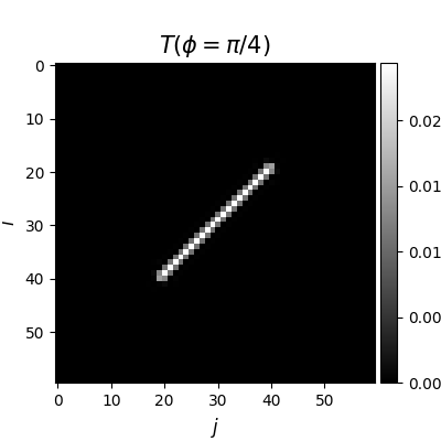
kernel = mr.streak_convolution_kernel([1.0, 1.0], 30)
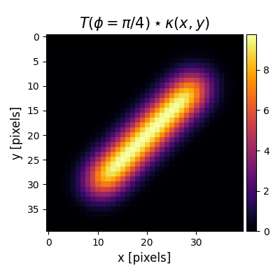
res = mr.convolve_with_kernel(gaussian_pattern, kernel)

Let’s look at the volume of both distributions

print(f'Gaussian volume: {np.sum(gaussian_pattern):.4f}')

Gaussian volume: 2105.0935

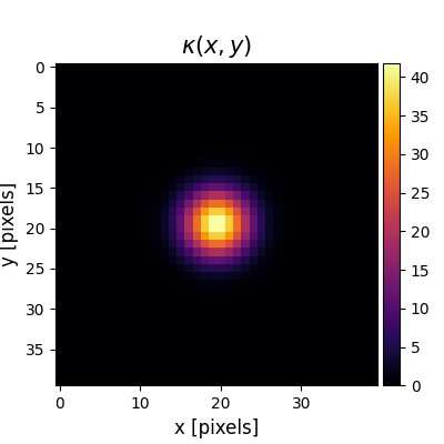
Visualize the Airy disk on the CCD grid

plt.figure(figsize=(4, 4))
plt.imshow(
    gaussian_pattern,
    cmap='inferno',
)
mrv.texit('$\kappa(x,y)$', 'x [pixels]', 'y [pixels]', grid=False)
plt.colorbar(cax=mrv.get_cbar_ax())
plt.clim(0, np.max(gaussian_pattern))

plt.figure(figsize=(4, 4))
mrv.texit('$T(\phi=\pi/4)$', '$j$', '$i$', grid=False)
plt.imshow(kernel, cmap='gray')
plt.colorbar(cax=mrv.get_cbar_ax())

plt.figure(figsize=(4, 4))
plt.imshow(res, cmap='inferno')
mrv.texit('$T(\phi=\pi/4) \star \kappa(x,y)$', 'x [pixels]', 'y [pixels]', grid=False)
plt.colorbar(cax=mrv.get_cbar_ax())
plt.tight_layout()
plt.show()

• 
• 
•