Importance Sampling

Reducing the variance of Monte Carlo integration

import matplotlib.pyplot as plt
import numpy as np
import sympy as sp
from scipy.stats.sampling import TransformedDensityRejection

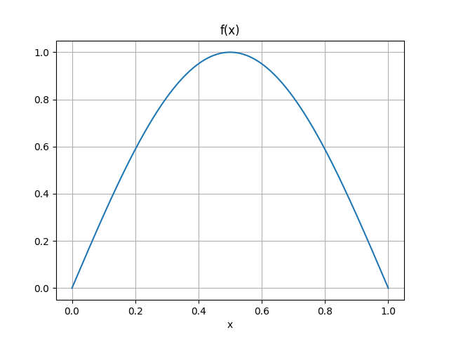
Let’s say we want to estimate the integral of an unknown function \(f(x)\)

x = sp.symbols('x')
f_symbolic = sp.sin(np.pi * x)
bounds = (0, 1)
f = sp.lambdify(x, f_symbolic)
xs = np.linspace(*bounds, 1000)

plt.plot(xs, f(xs))
plt.grid()
plt.title('f(x)')
plt.xlabel('x')
plt.show()

We can analytically compute the integral of this function

int_symbolic = sp.integrate(f_symbolic, (x, 0, 1))
print(f'The analytic integral is {int_symbolic:.4f}')

The analytic integral is 0.6366

A naive attempt at Monte Carlo integration would be to uniformly take samples of the function over the integral and average them

n = 10  # number of samples
f_of_x_naive = f(np.random.rand(n))
int_naive = f_of_x_naive.sum() / n
percent_error_naive = (int_naive - int_symbolic) / int_symbolic * 100

print(
    f'The naive Monte Carlo integral is {int_naive:.4f}, {percent_error_naive:.2f}% error'
)

The naive Monte Carlo integral is 0.4992, -21.58% error

The fundamental idea of importance sampling is that our Monte Carlo result will be better if we take samples from a distribution that looks like the true function, dividing each sample by its pdf likelihood. To accomplish this, let’s select a pdf that might help

class NewPdf:
    def pdf(self, x: float) -> float:
        # Note that this is slightly
        return -6 * x**2 + 6 * x

    def dpdf(self, x: float) -> float:
        return -12 * x + 6


dist = NewPdf()
pdf = TransformedDensityRejection(
    dist, random_state=np.random.default_rng(), domain=[0, 1]
)

Let’s try Monte Carlo integration again with the new pdf

xs_sample = pdf.rvs(n)
int_importance = (f(xs_sample) / dist.pdf(xs_sample)).sum() / n
percent_error_importance = (int_importance - int_symbolic) / int_symbolic * 100

print(
    f'The importance sampled integral is {int_importance:.4f}, {percent_error_importance:.2f}% error'
)

The importance sampled integral is 0.6347, -0.29% error

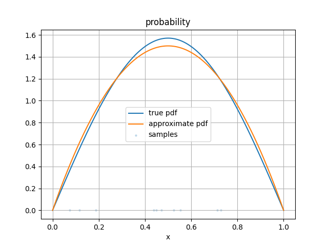
Let’s take a look at the points we sampled

true_pdf = f(xs) / int_symbolic
plt.figure()
plt.plot(xs, true_pdf)
plt.plot(xs, dist.pdf(xs))
plt.scatter(xs_sample, 0 * xs_sample, s=5, alpha=0.2)
plt.grid()
plt.title('probability')
plt.xlabel('x')
plt.legend(['true pdf', 'approximate pdf', 'samples'])
plt.show()